
Ryutarou Ohbuchi and Masaki Aono
Tokyo Research Laboratory, IBM Japan Ltd.
1623-14 Shimo-tsuruma, Yamato-shi, Kanagawa-ken, 242, Japan
ohbuchi@trl.ibm.co.jp and aono@trl.ibm.co.jp
In this paper, we describe a quasi-Monte Carlo (QMC) method, which employs deterministic low-discrepancy sequences (LDSs), to solve the global illumination problem. We first describe characteristics of two LDSs. Then, in a distribution ray-tracing setting, we show that the QMC integral with LDSs converges significantly faster than the Monte Carlo (MC) integral and about as fast as the stratified-Monte Carlo (SMC) integral with a typical pseudo-random sequence. Finally, we describe our adaptive error-bounded luminaire sampling (EBLS) method. The EBLS algorithm exploits two advantages of QMC; (1) convergence is faster and more accurate than MC, and (2) unlike SMC, samples can be added incrementally in small increments. Experiments showed that, given a budget of luminaire samples per image, the EBLS algorithm produces higher-quality images, especially in the penumbrae, than a method in which the numbers of samples per luminaire was predetermined.
CR Categories and Subject Descriptions: I.3.7 [Computer Graphics]: Three-Dimensional Graphics and Realism.
Additional Key Words and Phrases: ray-tracing, quasi-Monte Carlo integration, global illumination, luminaire sampling.
Many problems in computer graphics can be formulated as integrals. Global light-energy transfer can be expressed as an integral equation, which is sometimes called the rendering equation [8], and super-sampling screen pixels in the ray-tracing and the Z-buffer rendering algorithms are convolution integrals. The Monte Carlo (MC) integral is often used to compute these integrals, especially if the integrand is complex or higher-dimensional. (See elsewhere in [5, 9, 21] for more details on MC integral.)
The MC integral approximates an integral I(f) of a function
![]() by the following formula:
by the following formula:
The function is evaluated at N randomly selected points
![]() . While the MC method is quite effective, slow
convergence is an issue; the absolute value of the error has an
average magnitude of
. While the MC method is quite effective, slow
convergence is an issue; the absolute value of the error has an
average magnitude of ![]() .
.
Various methods have been employed to reduce the error of the MC method, such as importance sampling, stratified sampling, antithetic variates, and non-random sequences [8, 15, 23, 4]. These methods are mostly concerned with finding point sets that yield smaller integration errors. Importance sampling concentrates samples in the area where they are more effective by using a priori knowledge of the function. Stratified sampling tries to distribute samples evenly by subdividing the domain into subregions such as grids. Note that it is possible to combine some of these techniques, or to apply them adaptively. For example, uniformly distributed samples generated by stratification can be employed for importance sampling.
Since it has been observed that random point sets tend to take wasteful samples because of clumps and empty spots, error reduction by means of non-random point sets tries to use more uniformly distributed points. In computer graphics, non-random sequences generated by the n-rooks, Poisson disk, and other algorithms have been tried with some success [12, 17, 4]. However, these point sets have disadvantages. For example, the n-rooks can generate only very sparse sets of points, and the Poisson disk points are costly to generate.
An alternative to PRS is a class of deterministic (thus non-random) sequences called Low Discrepancy Sequences (LDSs). If LDSs are used to generate sample points for the MC method, the method is called quasi-Monte Carlo (QMC).
In computer graphics, LDS and QMC has not received much exposure in the past. LDSs have been applied to compute pixel intensity values by quasi-randomly perturbing the sub-pixel sample locations in the 2D screen coordinate space [6, 17]. Sampling in screen space is necessary in antialiased image generation using, for example, Z-buffer or eye-ray tracing methods. [6] compared Poisson, Poisson disk, regular grid, N-rooks, jittered, as well as Halton, Hammersley, and scrambled Halton point sets in terms of their performance for screen pixel sampling. [4] include a good discussion on various sampling techniques, including a brief mention of LDSs and summary of [12] which compared a Zaremba point set with several other sample point sets.
There are a few examples of QMC applied to solve global illumination problem. Heinrich and Keller [7] solved global illumination problem through particle tracing by using LDS. While details of their algorithm is not clear from the paper, it appears to be similar to the one described by Keller in his paper [10]. [7] concludes by experiments that the errors of the irradiance values of triangular patches in the test scene computed by using Hammersley point set was the smallest among the alternatives he tried. Keller [10] applied LDS to a radiosity methods that exchanges energy by MC (or QMC) ray-tracing among triangular patches. [10] show experimentally that the QMC performs slightly better than MC with pseudo-random sequences (PRSs). In ray-tracing setting, Shirley [20] describes importance sampling methods for various types of luminaire and a scheme to handle a large number of luminaires in a scene by treating multiple luminaires as a single irregularly shaped luminaire.
In this paper, we advocate the use of LDSs for solving integral equations in the global illumination problem. First, we briefly discuss characteristics of LDSs, Sobol' and Halton sequences. We then apply QMC in eye-ray tracing setting to compute contribution from direct luminaire and compares performance of QMC with the MC with PRS and stratified-MC (SMC) method with stratified-PRS (SPRS). An adaptive sample termination algorithm called error bounded luminaire sampling (EBLS) is described next. The EBLS is applicable to MC as well as QMC. However, the EBLS works best with QMC for it exploits (1) QMC's faster and more accurate convergence than MC, and (2) QMC's ability to add samples incrementally. SMC is not suited for adaptive sample termination with incremental addition of samples. Experiments showed that the QMC with EBLS produces higher-quality images than those generated by MC, QMC alone, and MC with EBLS.
The QMC method uses a formula which is formally identical to that of the MC method, except that the points used for evaluating the function are generated deterministically. Unlike the MC method, the QMC method has a deterministic error bound, and the accuracy of the integral is generally significantly better than in the MC method. (Note that QMC has certain restrictions compared to the MC method; MC is applicable to l2 space of functions, while QMC is applicable to integrand with bounded variation.)
The deterministic sequences used in the QMC method, LDSs, are designed
to have low discrepancy[14]. Discrepancy
is a measure of the uniformity of distribution of finite point
sets. Informally, it is error in an estimate of the volumes of a unit
cube, which is computed as the proportion of points in a subset of the
unit cube. Various discrepancy measures can be defined according to the
definition of the the subsets and the norm used. An LDS has a minimum
discrepancy of ![]() for a large number of points N
and a dimension d. While there are several variations, an error bound
for the QMC method is
for a large number of points N
and a dimension d. While there are several variations, an error bound
for the QMC method is ![]() [14, 13]. This bound suggests a potentially faster
convergence than in the MC method.
[14, 13]. This bound suggests a potentially faster
convergence than in the MC method.
LDSs include the Hammersley, Halton, Sobol', Faure, generalized Niederreiter and other sequences [14, 13, 22]. Of these, the Hammersley sequence has the deficiency that it is not possible to incrementally add points without discarding the points already generated. This deficiency matters when one tries to increase number of samples incrementally, for example, to sample to convergence. We chose the Sobol' and Halton sequences for the studies described in this paper. The generator for the Sobol' sequence is based on the program in [15], and the algorithm for Halton sequence is described in [14] and others. Description of Hammersley, Faure, and Generalized Niederreiter sequences are found in [14, 22].

Figure 1: Points 1 to 16 generated by PRS, SPRS, Sobol', and
Halton sequences. SPRS stratified the domain into ![]() strata.
strata.
Figure 1 shows plots of the first 16 points
generated in 2D plane by four methods: (a) a pseudo-random sequence
(PRS), (b) a stratified PRS (SPRS), (c) a Sobol', and (d) a Halton
sequence. As the PRS, we used drand48(), which has better
statistical properties as a pseudo-random sequence than the infamous
rand() in standard C libraries. For the SPRS, a 2D domain was
divided into ![]() and points were picked in each subdomain by a
pair of
and points were picked in each subdomain by a
pair of drand48() sequences.
Clumping and empty region is clearly seen in the points generated by the
PRS. Points generated by SPRS, Sobol' and Halton are more evenly
distributed. In terms of computational speed, in our experiment, the
Sobol' sequence was the fastest, taking about ![]() per-2D point,
while the PRS (
per-2D point,
while the PRS (drand48()) took ![]() and the Halton took
and the Halton took
![]() on our workstation (with an xlc compiler and the AIX 4.1.4
operating system running on a 100 MHz PowerPC 604).
on our workstation (with an xlc compiler and the AIX 4.1.4
operating system running on a 100 MHz PowerPC 604).
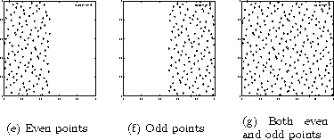
Figure 2: Even points (a) and odd points (b) generated by Sobol' as a
series of 2D points. Even and odd points fills only a half of the
domain. All the points covers entire unit square evenly (c).
It should be noted that the QMC method with LDSs is not a panacea and care must be taken in its application. One of its problems is periodicity. For example, if a 2D point sequence is generated, the first dimension (horizontal axis of the plots in Figure 2) of the Sobol's sequence generated by the code in [15] alternates between the upper and the lower half of the interval [0,1]. This can be clearly seen in Figure 2 (a) and (b), which plotted even and odd points generated by Sobol' sequence, respectively. When the points are combined, the points fills the rectangle evenly (Figure 2(c)).
Periodicity also appears in LDS when a higher-dimensional sequence is generated. Both Halton and Sobol' sequences in higher dimensions require fairly large numbers of points to populate the interval [0,1]. For example, [13] shows a 2D plot of points that paired dimensions 27 and 28 of their Sobol' sequence generator, which exhibits checkerboard-like pattern when the first 8192 points were plotted. It took the total of 16384 points before the distribution of points looked uniform. The behavior of a point sequences in higher dimensions is important if indirect illumination is considered, in which multiple bounces of light increase the dimensionality of the integral.
The rendering equation for global illumination [8] is an example of complex, higher-dimensional integrals. (See elsewhere [2, 4] for detailed discussion of the global illumination and the rendering equation.) The MC and QMC are used to solve the rendering equation in both the ray-tracing [3, 8, 12, 1, 16, 18, 20, 23] and in radiosity [19, 10] framework.
We wish to compute radiance L from the point ![]() in the
direction
in the
direction ![]() (see Figure 3). This radiance
results from the contribution of luminaire S reflected by
bidirectional reflectance distribution function (BRDF)
(see Figure 3). This radiance
results from the contribution of luminaire S reflected by
bidirectional reflectance distribution function (BRDF) ![]() and
emission
and
emission ![]() from the point
from the point ![]() .
. ![]() is the incoming
radiance from the point
is the incoming
radiance from the point ![]() on the luminaire. V is the
geometry term, which is 1 if
on the luminaire. V is the
geometry term, which is 1 if ![]() is directly visible from
is directly visible from
![]() and 0 otherwise.
and 0 otherwise. ![]() (
( ![]() ) is the angle
) is the angle ![]() (
( ![]() ) makes with normal
) makes with normal ![]() (
( ![]() ). If indirect
light transport is to be computed, the following equation is applied
recursively multiple times.
). If indirect
light transport is to be computed, the following equation is applied
recursively multiple times.
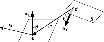
Figure 3: Illustration of direct illumination of point x by luminaire S.
We assume that the radiance ![]() is constant over
the surface of the luminaire. We also assume that there is no emission
from the point
is constant over
the surface of the luminaire. We also assume that there is no emission
from the point ![]() . Equation 2 becomes
. Equation 2 becomes
We apply the MC or QMC method to choose the point ![]() .
The outgoing radiance L can be computed by approximating the area
luminaire with N point luminaires.
.
The outgoing radiance L can be computed by approximating the area
luminaire with N point luminaires.
In the MC method, sample points ![]() are generated by a
pair of random numbers
are generated by a
pair of random numbers ![]() and
and ![]() in the interval [0,1].
In reality, a PRS is used for the MC method due to the lack of
real random sequence. For the QMC method, a LDS is used in place
of a PRS.
in the interval [0,1].
In reality, a PRS is used for the MC method due to the lack of
real random sequence. For the QMC method, a LDS is used in place
of a PRS.
We compared the performance of the four methods, which included both MC and QMC, by using direct luminaire sampling as an example for experiments.
We solved equation (4) for a single bounce of light
from a luminaire, i.e., for the direct illumination, by using the
distribution (eye-) ray-tracing algorithm . For BRDF, we used
mirror-reflection, Phong's specular, and complete diffuse terms.
A sample point ![]() on a square luminaire is generated,
on a square luminaire is generated,
![]() where
where ![]() are 3D orthonormal vectors that span the square and
k is the length of an edge of the square. For the SMC method, the same
procedure was repeated for each stratum.
are 3D orthonormal vectors that span the square and
k is the length of an edge of the square. For the SMC method, the same
procedure was repeated for each stratum.
Figure 4 and Figure 5 shows images
generated by the four methods by using 16 and 36 samples, respectively,
to sample a luminaire. The scene contained a ground plane, a sphere, and
a square luminaire. The images ( ![]() pixels) are generated
by casting one eye-ray per pixel (i.e., without super-sampling). Each
ray is traced from a pixel until it intersects a surface at a point
pixels) are generated
by casting one eye-ray per pixel (i.e., without super-sampling). Each
ray is traced from a pixel until it intersects a surface at a point
![]() , from which rays are cast to sample 16 points (or 36 points)
on the luminaire. The 16 sample points on the luminaire were generated
by the same four methods as in the experiment described in
Section 2 (see Figure 1).
, from which rays are cast to sample 16 points (or 36 points)
on the luminaire. The 16 sample points on the luminaire were generated
by the same four methods as in the experiment described in
Section 2 (see Figure 1).
We conducted informal evaluation of image quality by asking several colleagues.
For the images generated by 16 samples, Everybody picked the image generated by QMC with Halton as the best quality image. Visual qualities of the images generated by Sobol' and stratified-MC (SMC) were close. Some picked Sobol', while the others picked SMC. Those who picked SMC pointed out systematic artifacts in the image generated by Sobol'. All the subjects picked the image produced by MC as the worst.
The results are similar for the images generated with 36 samples, although the images by SMC, Sobol' and Halton had become more difficult to distinguish. Systematic artifacts that existed in the images by Sobol' and Halton had almost (but not quite) disappeared at this number of samples.
Figure 6 compares the convergence of intensity at a
ray-object intersection point ![]() illuminated by a square
luminaire without any blocker, for MC with PRS and QMC with the Sobol'
and Halton sequences. Each graph plots 10 runs at the same point
illuminated by a square
luminaire without any blocker, for MC with PRS and QMC with the Sobol'
and Halton sequences. Each graph plots 10 runs at the same point ![]() on an object (not at a screen pixel). (SMC is not included in the
figure since the SMC method does not allow incremental increase of
number of samples.)
on an object (not at a screen pixel). (SMC is not included in the
figure since the SMC method does not allow incremental increase of
number of samples.)
In this experiment, the convergence of QMC with the Halton sequence appears to be the fastest, followed by QMC with the Sobol' sequence, while MC with PRS was the slowest. The accuracy of the conversion seems to follow the same order; QMC with the Halton sequence appears to converge to the most accurate value, followed by QMC with the Sobol' sequence and finally by MC with PRS.
We repeated this experiment under different conditions, for example, with luminaires of several different shapes and with different initialization parameters (e.g., Sobol's generator polynomial) for the LDSs. In some cases, QMC with the Sobol' sequence converged as fast or faster than QMC with the Halton sequence. MC with PRS, however, converged the slowest in the every cases we tried.

Figure: Images of the sphere with the shadow are generated by taking
16 samples on the square luminaire by using the PRS, SPRS, Sobol', and
Halton point sets.
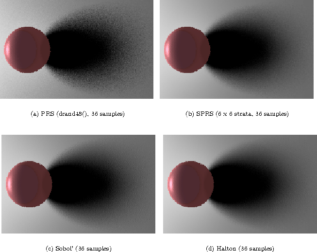
Figure: Images of the sphere with the shadow are generated by taking
36 samples on the square luminaire by using the PRS, SPRS (6 x 6
strata), Sobol', and Halton point sets.
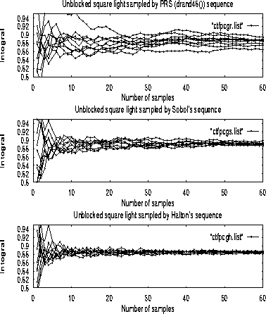
Figure 6: Convergence of MC and QMC integrals that sampled unblocked
square luminaire. The QMC by LDSs Sobol' and Halton sequences
converge much faster than the PRS drand48().
We quantified ``quality'' of images computed above by computing an error
measure. We compared the intensity values in the screen space of a
``reference'' image with those the images generated by the four sampling
methods with a small number (16) of samples per luminaire. We used
root-mean-square distance of intensities of all the pixels in the images
as the measure. Error ![]() of image intensity x and y of
the size pq = M pixels is computed by;
of image intensity x and y of
the size pq = M pixels is computed by;
where the RMS distance of the pixel intensity
Figure 7 compares the error in the images generated by
point sets due to PRS, SPRS, Sobol' and Halton, shows the RMS errors
normalized by the worst case value, PRS with 4 samples. For the SPRS,
the domain is fully stratified, i.e., one 2D point by PRS is dropped in
each stratum. The reference image is computed by taking ![]() luminaire samples per ray-object intersection, by MC. (To make sure the
``reference'' by MC is a good approximation of a reference image, we
have compared it with the images computed by SMC and QMC methods with
luminaire samples per ray-object intersection, by MC. (To make sure the
``reference'' by MC is a good approximation of a reference image, we
have compared it with the images computed by SMC and QMC methods with
![]() samples.)
samples.)
It can be clearly seen in the graph that the RMS error decreases faster with the SMC and QMC methods than the MC method. At 81 samples, the error in the MC method is almost three times as large as the errors in the SMC and QMC methods. Of the three methods that performed well, Halton performed the best, followed by SPRS, and then by Sobol.
Theoretical error bounds for SMC and QMC are asymptotically close, and the experimental results in the Figure 7 supports this. An advantage of QMC is that it is easy to incrementally add small number of sample points, for example, until a certain error criteria is met. Such addition of samples in small increment is difficult with the SMC. A disadvantage of QMC compared to SMC is the artifacts in the image due to the deterministic nature of the LDSs, especially at smaller number of samples.
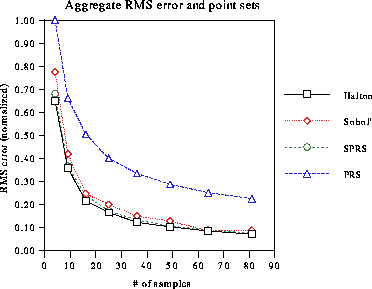
Figure 7: Convergence of MC and QMC integrals that sampled unblocked
square luminaire. The SMC, and QMC by LDSs Sobol' and Halton sequences
converge much faster than the MC by PRS drand48().
Typically, a luminaire sampling method in a ray-tracer has a fixed (user
specified) number of samples per area luminaire. Such a method
frequently over-samples in some places and under-samples at the others.
We have developed the Error-Bounded Luminaire Sampling (EBLS)
algorithm that adaptively concentrates luminaire samples where they are
needed based on convergence estimates. The convergence criterion of EBLS
relies solely on the knowledge of estimated irradiance value at the
ray-object intersection point ![]() . For example, the criterion does
not take spatial variation of irradiance into consideration.
. For example, the criterion does
not take spatial variation of irradiance into consideration.
The EBLS can be applied to luminaire sampling by either MC or QMC. However, EBLS works better if combined with the QMC by taking advantage of the QMC's faster and more accurate convergence. EBLS is suited more to QMC than SMC, since QMC allows sample points to be added incrementally in much smaller increments than in SMC.
Convergence check can be performed by various methods. However, since
the convergence test is performed frequently, its overhead must be
small. If the overhead for the convergence test is large, it might be
less expensive to simply over estimate the necessary number of
samples. We have used the the average of incoming
irradiance at point ![]() , which must be computed
anyway to obtain an estimate of the integral. Other possible measure for
the termination criterion include, for example, variance.
Note that the luminaire sampling takes place in the world space so that
we could not use the criterion based on spatially local contrasts in the
screen space, as employed in Mitchell [11] and Schlick
[16].
, which must be computed
anyway to obtain an estimate of the integral. Other possible measure for
the termination criterion include, for example, variance.
Note that the luminaire sampling takes place in the world space so that
we could not use the criterion based on spatially local contrasts in the
screen space, as employed in Mitchell [11] and Schlick
[16].
The EBLS algorithm increases the number of samples n by the increment
t. Our convergence check compares the previous intensity estimate of
the color vector
![]() at point
at point ![]() computed with
(n-t) samples and the last intensity estimate at the same point
computed with
(n-t) samples and the last intensity estimate at the same point
![]() computed with n samples. The sampling
stops if all the conditions
computed with n samples. The sampling
stops if all the conditions ![]() ,
,
![]() , and
, and ![]() hold.
The larger the parameter t the more accurate the result, but the
chances of wasting samples increase.
hold.
The larger the parameter t the more accurate the result, but the
chances of wasting samples increase.
Figure 8 compares four images generated by EBLS and
fixed sampling (FS). The scene contained four objects visible in the
image, the floor, and a square luminaire. The four cases are: (a) MC
with FS, (b) MC with EBLS, (c) QMC (Sobol') with FS, and (d) QMC
(Sobol') with EBLS. In the EBLS cases, t=5 and
![]() . In the FS cases, at each point, the luminaire is
sampled by a predetermined number of points m. We first computed the
image by using case (d), and tried to use an approximately equal but not
smaller number of rays for case (c) by choosing a fixed number m of
samples per point
. In the FS cases, at each point, the luminaire is
sampled by a predetermined number of points m. We first computed the
image by using case (d), and tried to use an approximately equal but not
smaller number of rays for case (c) by choosing a fixed number m of
samples per point ![]() . We then used the same EBLS termination
criterion as (d) for case (b), and tried to use an approximately equal
but not smaller number of rays for case (a). The total number of rays in
these images, which include reflecting rays with depths of up to 3, were
as follows: (a) MC with FS:
. We then used the same EBLS termination
criterion as (d) for case (b), and tried to use an approximately equal
but not smaller number of rays for case (a). The total number of rays in
these images, which include reflecting rays with depths of up to 3, were
as follows: (a) MC with FS: ![]() rays, (b) MC with EBLS:
rays, (b) MC with EBLS:
![]() rays, (c) QMC with FS:
rays, (c) QMC with FS: ![]() rays, and
(d) QMC with EBLS:
rays, and
(d) QMC with EBLS: ![]() rays. Execution time is
roughly proportional to the number of rays.
rays. Execution time is
roughly proportional to the number of rays.
The EBLS clearly improved image quality, especially of penumbrae, over FS, in both the MC and QMC methods. Dark dots in the penumbrae, which are the points where most of the luminaire-sampling rays were ``unfortunately'' blocked from reaching the luminaire by objects, are much less visible in images generated with EBLS than their counterparts with FS. This is because EBLS adaptively concentrates rays in the area of high variance - in this case, the penumbra. Of the four methods, the QMC with EBLS produced the best quality result in the least amount of time. As expected, EBLS was less effective if applied to MC than to QMC method. Even if EBLS was used, MC often converged to inaccurate values, thereby producing grainier image than the image by QMC with EBLS. The EBLS method was made practical by the faster and more accurate convergence of QMC with LDS.
In this paper, we discussed a quasi-Monte Carlo (QMC) method with low-discrepancy sequences (LDSs) for solving global illumination problems in ray-tracing setting. First, we discussed characteristics of LDSs. Then, using the direct luminaire sampling in the distribution ray-tracing framework as an example, we showed by experiments that the QMC method can outperform the classical Monte Carlo (MC) method in terms of speed and accuracy of convergence. The QMC is about as effective as stratified-MC method in terms of convergence speed and accuracy. However, QMC has an advantage over SMC in that the number of samples can be increased easily in small increment without introducing significant sampling bias. As a disadvantage, with lower number of luminaire samples, QMC could introduce systematic artifacts that are more visible than the random error introduced by SMC. However, the artifacts due to QMC disappear as the number of samples is increased. We also described an error-bounded, ray-by-ray adaptive termination algorithm for luminaire sampling. The adaptive sample termination algorithm works well with either MC or QMC (but not SMC) luminaire sampling. However, it works best if applied to QMC luminaire sampling, by taking advantage of QMC's fast convergence and ability to add samples incrementally. The experiment showed that, if total numbers of rays per images are identical, the error-bounded termination of luminaire sampling could produce higher-quality images than the method with a predetermined number of samples per luminaire.
In the future, we would like to try combining the QMC method with other variance reduction measures such as importance sampling. We would also like to investigate the application of a new class of LDSs, such as generalized Niederreiter sequences [14, 22], which potentially have better properties, especially in generating sequences with higher dimensions. Since the dimension of the integral increases with each bounce of light in the ray-tracing framework, good behavior of LDSs in higher dimensions could become crucial.

Figure 8: Images rendered with fixed number of luminaire samples, and
with error-bounded sample termination, by using PRS.
Acknowledgments
We thank Mr. A. Tajima of IBM Tokyo Research Laboratory for providing us with the Halton sequence generator.